Lossy Image Compression with Dithering
Last year I took an elective on Computer Graphics (course notes) where I learned about OpenGL shaders, and image compression algorithms.
One of the algorithms I learned about was Floyd–Steinberg dithering.
Sometimes when storing an image, we want to compress it lossily: we create a new version of it that loses a part of the information and quality, but is significantly smaller in filesize.
One way of achieving this, is using a reduced palette. The GIF format does this, for instance, by limiting the available colors in a single file to 256.
Mapping colors to the most similar one available in a palette is called vector quantization, since we are effectively subdividing the whole color space into regions and assigning one color to each.
Mapping pixels from the entire color space (which has 256\^3 possibilities) to a reduced set of values can generate a problem, though: regions of neighboring pixels tend to have similar colors, and the most straightforward way of mapping them, where each pixel goes to the most similar color available in the reduced palette, will generate large regions of a single flat color in an image, producing artifacts. This looks quite ugly to human eyes.
Dithering aims to solve the problem of large flat areas by altering the colors of neighboring pixels after mapping one to a color from the palette. What’s novel about this method is that it carries over the difference between each pixel and its new in-palette assigned color, propagating it to its neighbors. This way, if for instance I map a pixel to a darker color from my palette, I will make the next neighboring pixels brighter to compensate in average, since I will end up nudging them closer to different elements from the palette. This system prevents artifacts that look like monochromatic flat areas and preserves nuance better.
However, since we will effectively be adding noise so the pixels in the surrounding region after changing each pixel, this will tend to increase entropy in the resulting image, making compression less effective. Generally we will need to evaluate the trade-off between image quality and compression.
The exact way the error is propagated is a bit arbitrary: just a convex distribution with most of it going to the neighbors below or to the right, and some in diagonal. What’s interesting is that this way we can take an image that has lots of different colors, and obtain one that has a reduced palette but keeps most of the information, at least perceptually.
Algorithm and Implementation Details
For this project, I implemented dithering in Python using numpy. The algorithm itself is simple, and I used the pseudocode from Wikipedia as a starting point.
All we do is:
- Move through all the pixels sequentially.
- Given the current pixel, map it to the closest color in the palette.
- Compute the difference between the old color and the new one.
- Add a percentage of that difference to each of the pixel’s neighbors.
Here is the Python code for it.
I solved the color lookup using scipy’s KDTree, but if you wanted to code everything from scratch you could just replace this with a linear search for the minimum distance element in the table (or use numpy’s argmin).
Choosing a Palette
We can choose the palette in different ways.
For these experiments I went for evenly spaced palettes. I built them adding every multiple of 255/k for a given k, in all possible combinations for R, G and B. RGB colors go from (0,0,0) to (255,255,255), so this way given a certain k, we can guarantee no color will have to be mapped to a new one farther away than 128/k from it in any component.
A smarter approach to build a palette of k colors may have been running K-means clustering over the image to find k centroids to use as colors, and then use those for a k-color palette. Or maybe just taking the most common color, removing all colors closer than a certain threshold to it, and then repeating those two steps k times.
Experiments and Results
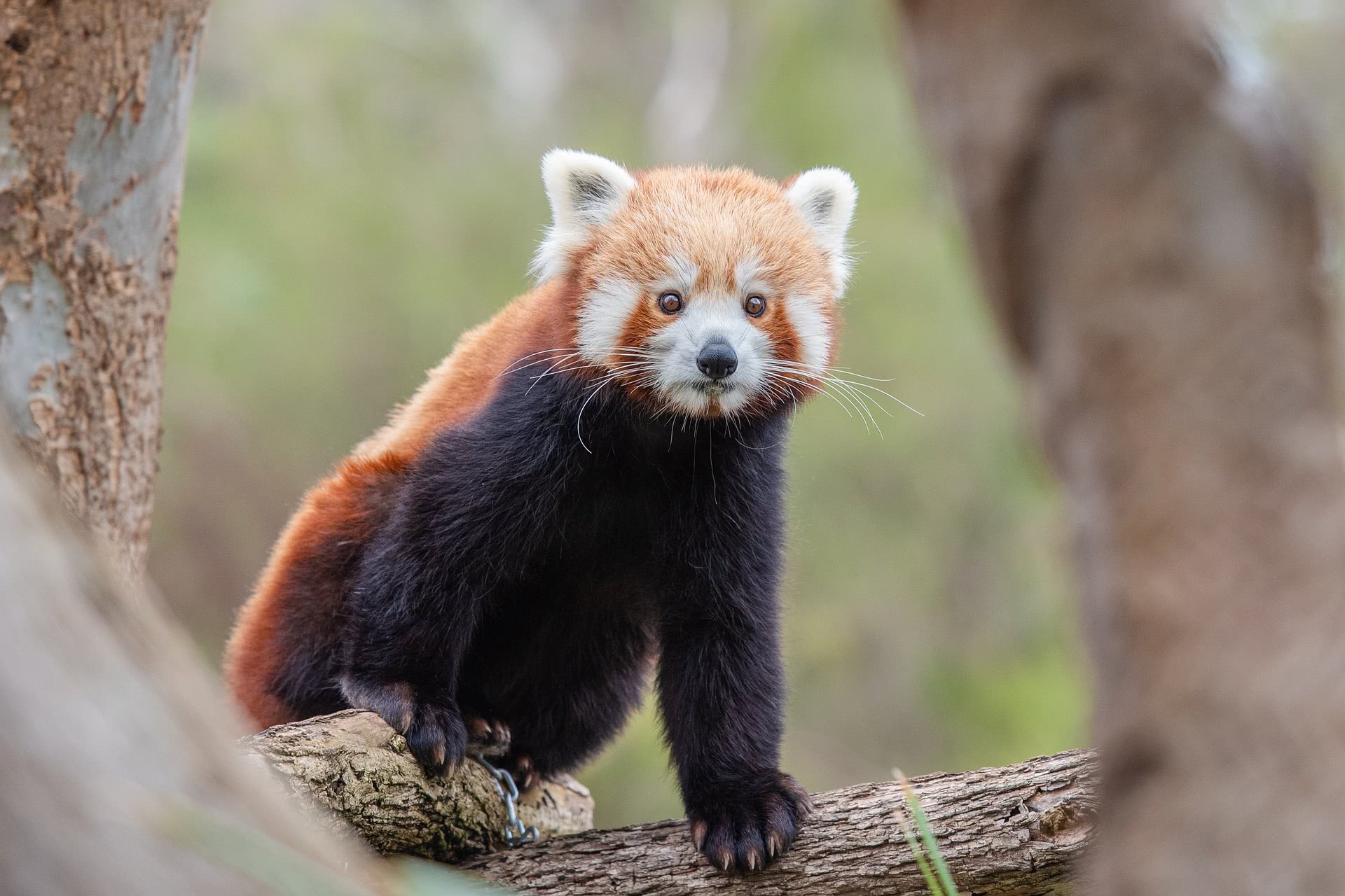
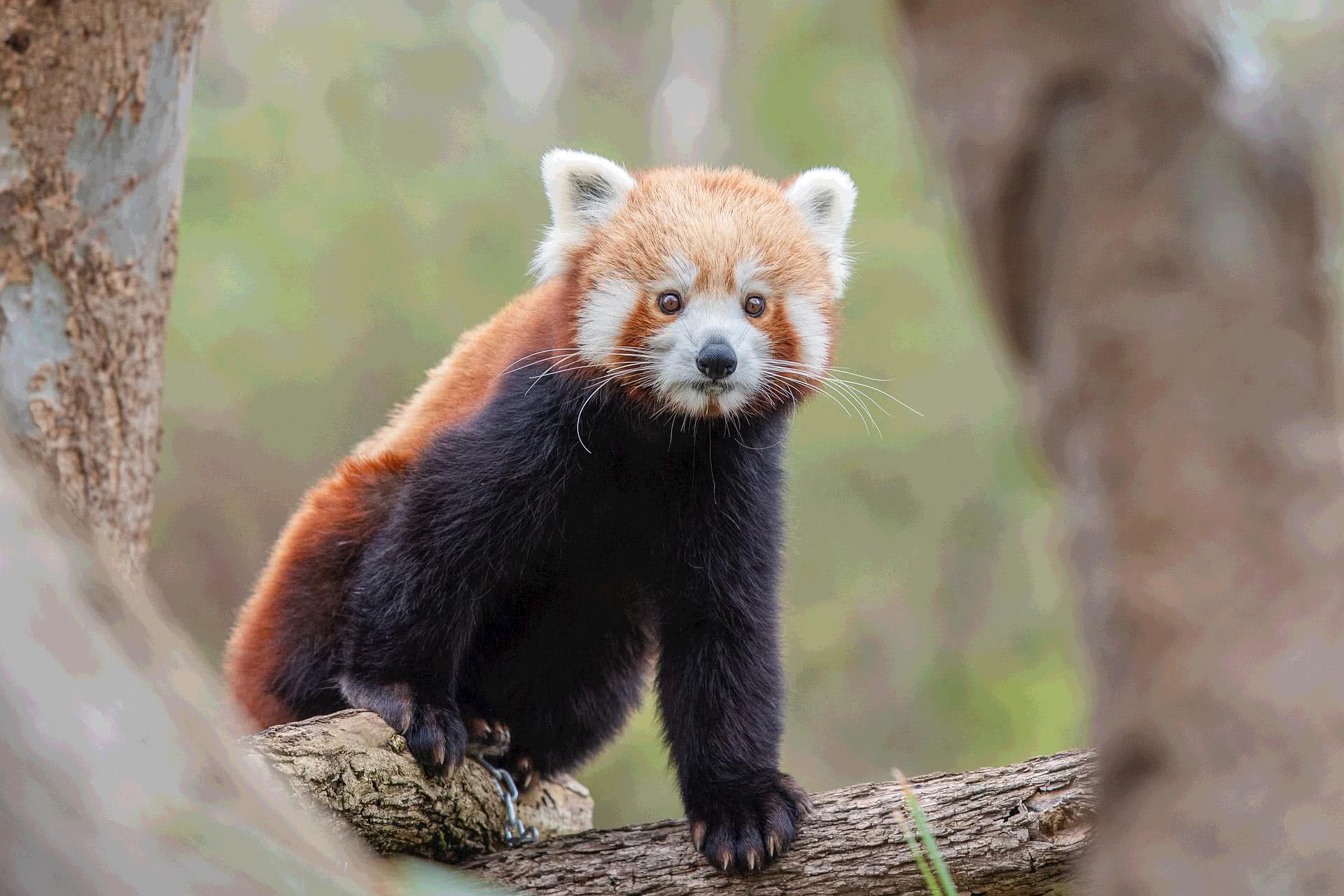
As an experiment to see how fast the algorithm was and how much smaller the file could get, I ran dithering compression on this image of a red panda (source: pixabay).
Here are the compressed versions after using palettes of evenly spaced colors (as described above) with k = 2, 4, 8 and 16. Note that for k=2, the palette is simple (only 0, 128 or 255 in each value of the color) and for k=16 we’re closer to representing every color (over 5000 different colors out of 256^3=~16M).
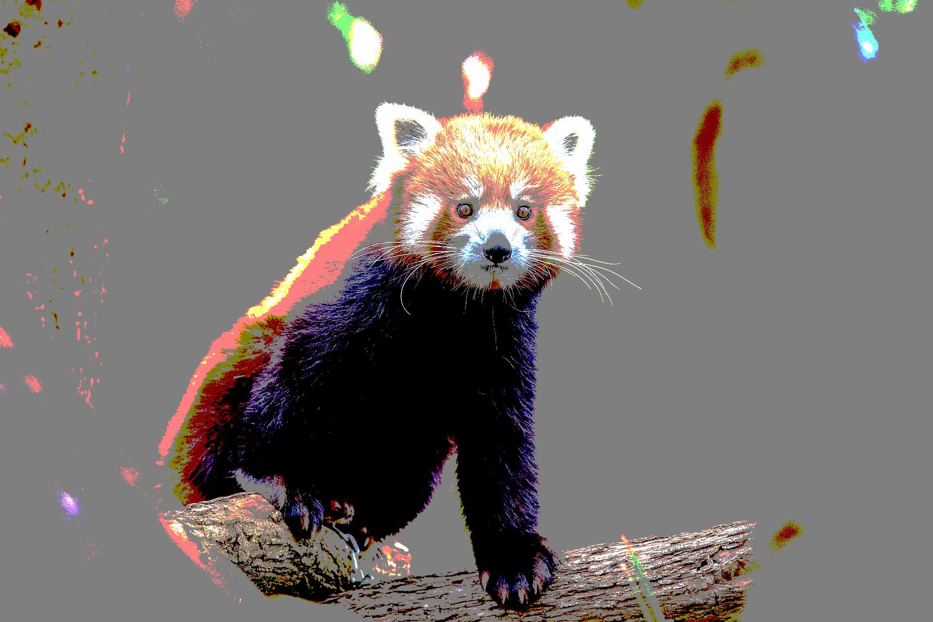
Compressed image with extremely small palette (k=2)
In this case, most of the background was converted to grey. The picture went from 580Kb to 264Kb in size, but at what cost.
We can see how the image loses less information as we increase palette size:
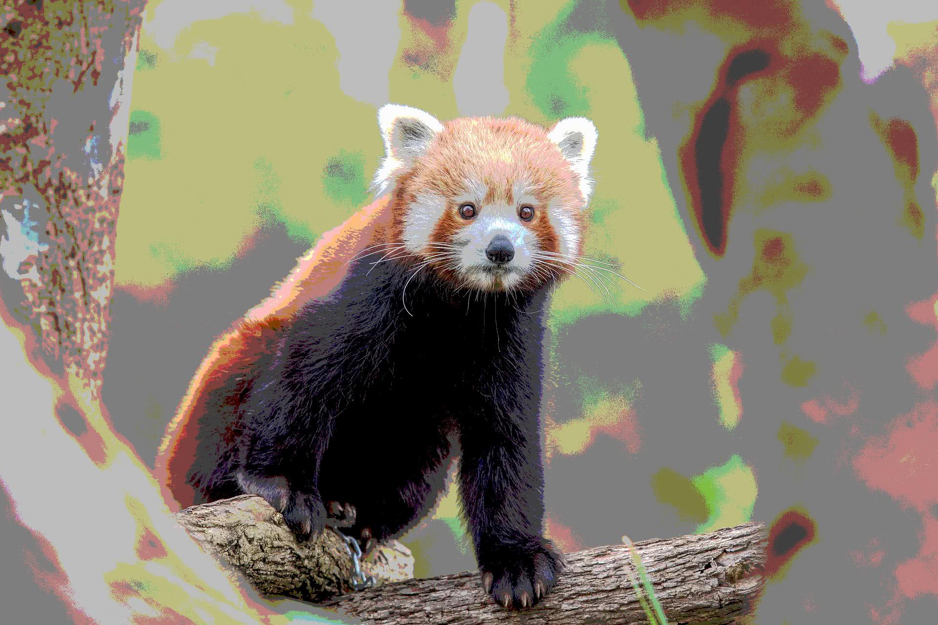
Compressed image with k = 4
Compressed image with k = 8
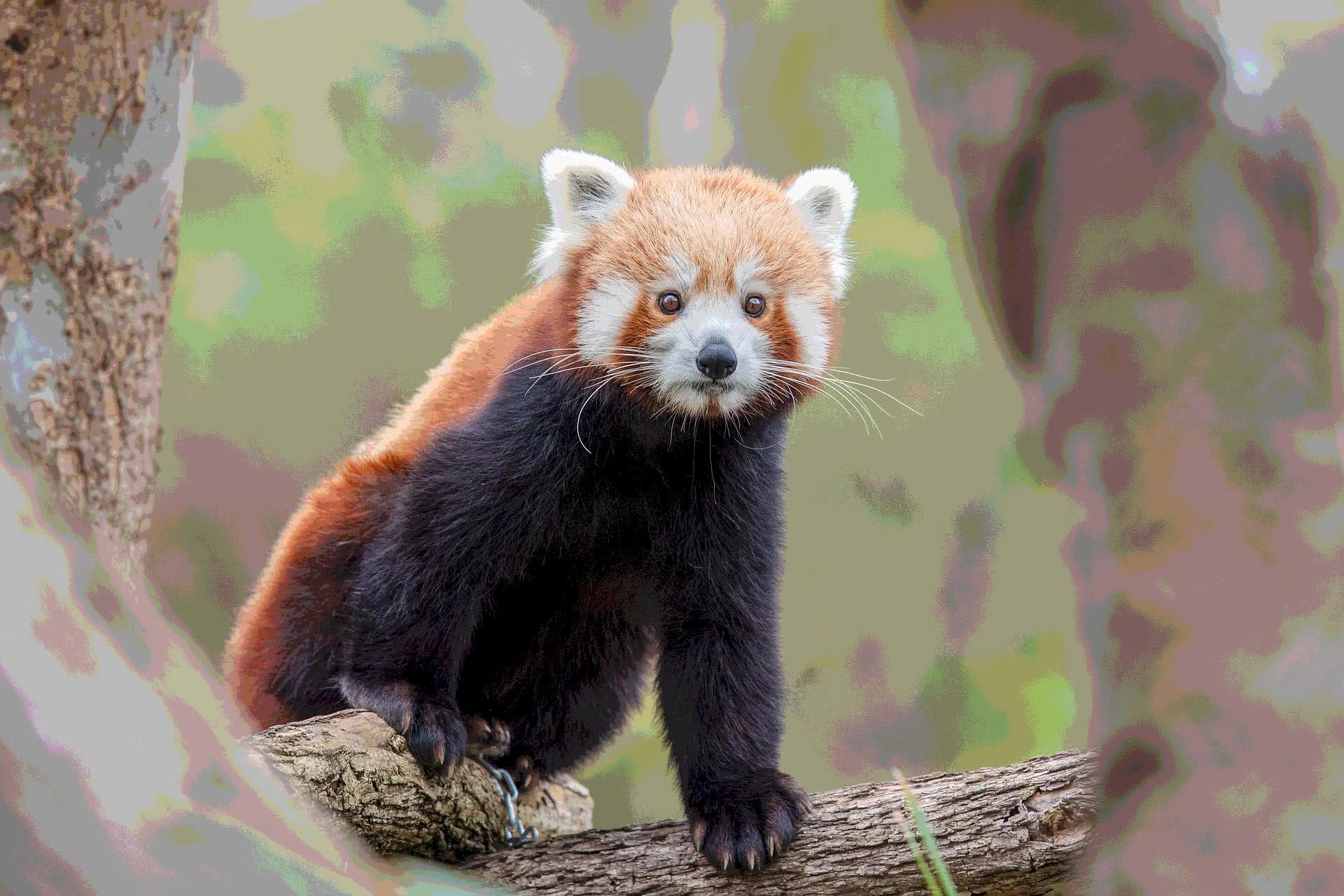
Compressed image with k = 16
The image with the biggest palette looks pretty similar to the original (except in the background details) but has a size of 344Kb. That’s a 40% reduction.
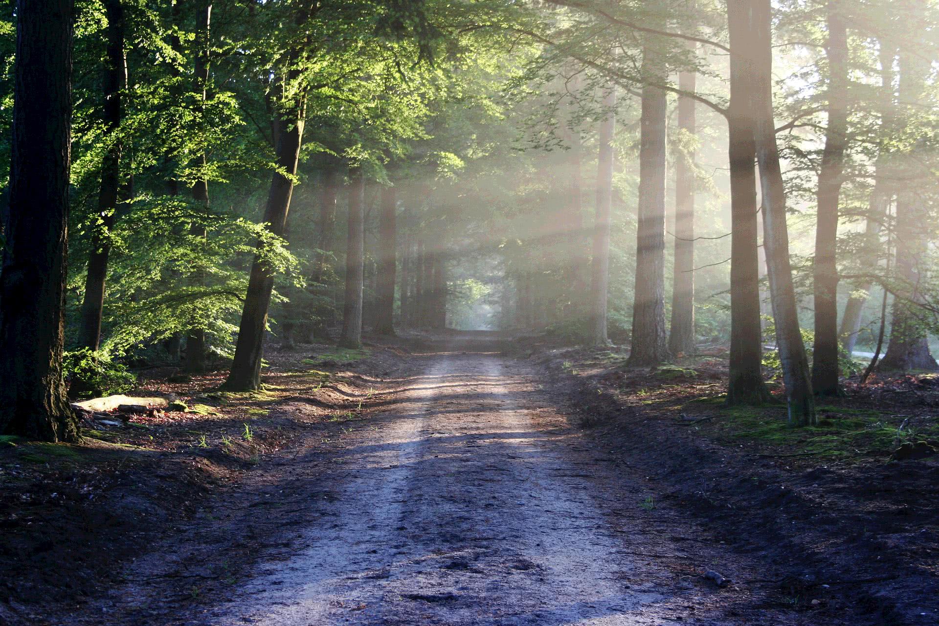
Just to make sure, let’s try a different image.
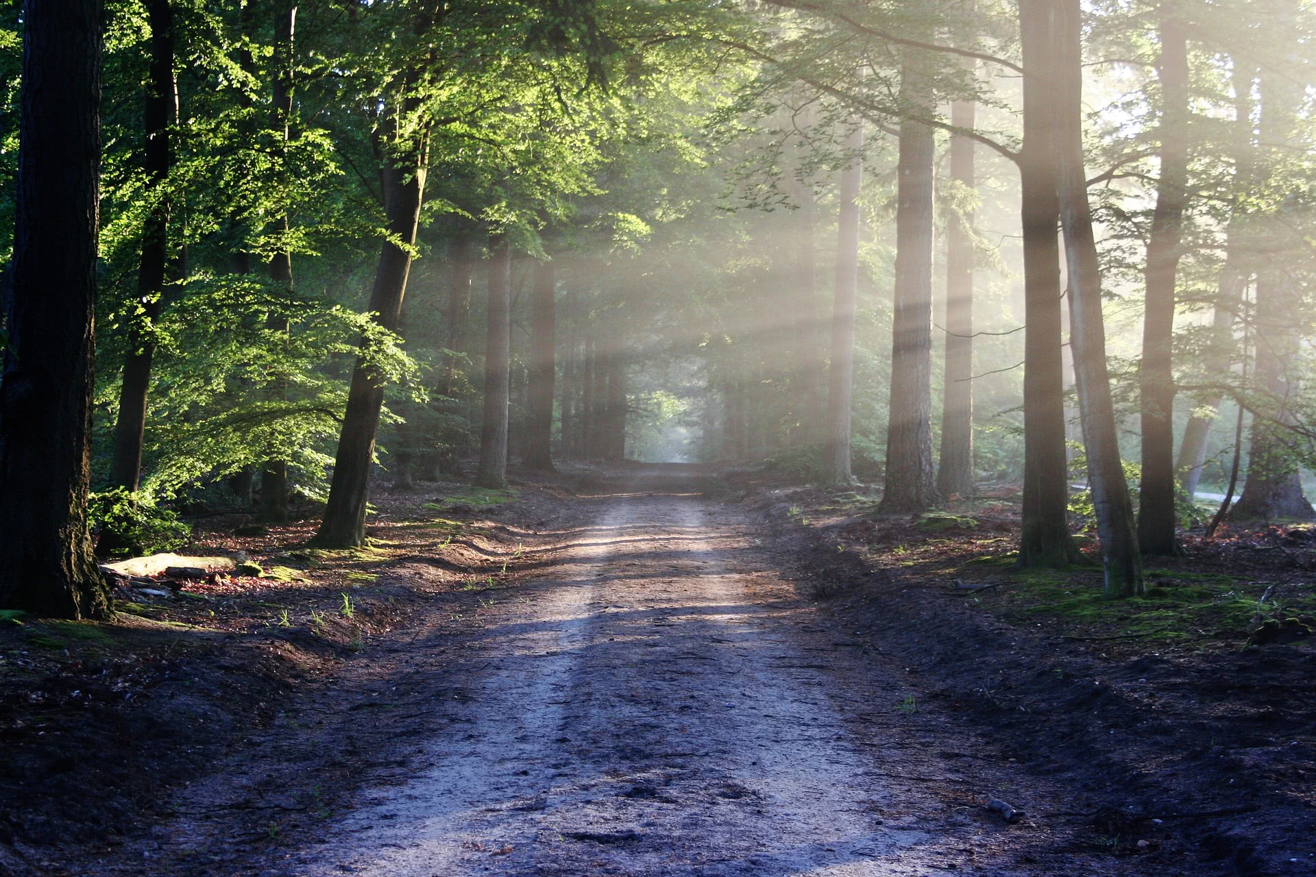
source: pixabay
Again with k=16 (palette of ~5800 colors), this is what we obtain:
This time, I’d say the image looks about the same. But now the size went down from 962Kb to 534Kb.
That’s a reduction of 41% for a difference that we mostly don’t notice.
Extending to .png
User @gakxd on Reddit remarks correctly that, since JPEG is a lossy format in itself, we can’t make such a direct conclusion from the reduction in size seen after applying dithering. In fact dithering may interact poorly with JPEG compression. Due to that, I thought it was worth repeating the experiment with a .png image. In this case I am using this site’s twitter card image, and compressing it with a palette of k=16 again (5800 colors).
Since .png is a lossless format, it will save the colors exactly the way this program leaves them, and we can compare results more directly this way. The only modifications I had to add to the program were for dealing with RGBA instead of RGB images, and my solution has simply been to leave the ‘A’ channel unchanged (keeping identical transparency) and only propagate errors forward if the A value is bigger than 0. I am not including the code itself as it would be pretty redundant.
Here are the results.


original image, image with a reduced palette (k=16)
Again, the images look pretty similar (only the fruits in the tree suffered a little from the compression), and this time the file size went from 160Kb to 92Kb, for a reduction of 42% again. And this time, we can appreciate exactly how the image changed, and know that all the gains were solely from the use of dithering, and no other changes to the image itself.
I am not sure what compression algorithms the PNG format uses so I’m not sure if reducing the palette and avoiding contiguous areas of the same color, which is what dithering does, will contribute possitively to them or not. I leave that for the community to discuss.
For fun, I tried the .png version on a bigger file (3.4MB) and it got to 885Kb with our k=16 palette. It’s even less than half the size now.

before and after
Conclusion
We made a simple image compressor that runs sequentially over an image’s pixels mapping them to their closest color in a reduced palette. This way we can constrain it to a smaller color-space and reduce its size significantly.
For most of the images tried, using a palette of 5800 colors represented a small perceptual difference in quality, but a 40% reduction in size.
I thought of maybe speeding up the program with parallel execution, but found the implementation a bit tedious. However I’m linking the paper for further reading, in case anyone is interested.
After further reading about compression, I wrote my notes in the data compression wiki article. I may do a follow up post explaining Huffman codes and the LZ77 algorithm for lossless compression.